Applying Brinson Model to a portfolio in 2022 with Python!

• full code in Colab
• Medium post(Chinese)

Intro

One of my classmate in Fudan told me that he had a great performance in HK stock market in 2022, is it true? Where was his performance come from?

Let's find out with Brinson Model.

Before we started calculation, we have picked Heng Seng Index as our benchmark(cuz our portfolio traded at HK stock market). We also collected the four types of necessary data, they are...

• return of each sector of Benckmark
• weight of each sector of Benckmark
• return of each sector of Portfolio
• weight of each sector of Portfolio

Now we let our Python 🐍 do the job.

Calculation

First import packages

import matplotlib.dates as mdates
import matplotlib.pyplot as plt
from google.colab import files, drive
import matplotlib as mpl
import pandas as pd
import numpy as np

try:
  !gdown --id 1fsKERl26TNTFIY25PhReoCujxwJvfyHn
  zhfont = mpl.font_manager.FontProperties(fname='SimHei .ttf') # make mpl show chinese
except:
  pass

then we import the data.

benchmark_and_portfolio = pd.read_excel('benchmark_and_portfolio.xlsx')
benchmark_and_portfolio['excess_return'] = (benchmark_and_portfolio.r_portfolio - benchmark_and_portfolio.r_benchmark).round(5)

then we can do the calculation, here we use the BHB Model, instead of BF Model.

brinson_model = pd.DataFrame(columns=['date', 'sector', 'allocation_effect', 'selection_effect', 'interaction_effect', 'excess_return'])
brinson_model['date'], brinson_model['sector'] = benchmark_and_portfolio['date'], benchmark_and_portfolio['sector']

#allocation effect (bhb model)
brinson_model['allocation_effect'] = ((benchmark_and_portfolio['w_portfolio']-benchmark_and_portfolio['w_benchmark'])*(benchmark_and_portfolio['r_benchmark']))
brinson_model.loc[brinson_model['sector']=='Total', ['allocation_effect']] = brinson_model[brinson_model['sector']!='Total'].groupby('date').sum(['allocation_effect']).reset_index()['allocation_effect'].to_list()

#selection effect
brinson_model['selection_effect'] = ((benchmark_and_portfolio['w_benchmark'])*(benchmark_and_portfolio['r_portfolio']-benchmark_and_portfolio['r_benchmark']))
brinson_model.loc[brinson_model['sector']=='Total', ['selection_effect']] = brinson_model[brinson_model['sector']!='Total'].groupby('date').sum(['selection_effect']).reset_index()['selection_effect'].to_list()

#interaction effect
brinson_model['interaction_effect'] = ((benchmark_and_portfolio['w_portfolio']-benchmark_and_portfolio['w_benchmark'])*(benchmark_and_portfolio['r_portfolio']-benchmark_and_portfolio['r_benchmark']))
brinson_model.loc[brinson_model['sector']=='Total', ['interaction_effect']] = brinson_model[brinson_model['sector']!='Total'].groupby('date').sum(['interaction_effect']).reset_index()['interaction_effect'].to_list()

# excess return
brinson_model['excess_return'] = brinson_model[['allocation_effect', 'selection_effect', 'interaction_effect']].sum(axis=1)

# round to 5th digit
brinson_model = brinson_model.round(5)

# show
brinson_model

Now we get a beautiful Brinson Model DataFrame~

Before we further do the visualization, let's check our calculation with the excess_return data. Since the excess_return equals to

return of portfolio minus return of benchmark,

also equals to

allocation_effect add selection_effect add interaction_effect.

All we have to do is to verify this in our Brinson Model DataFrame.

# checking calculation
diff_of_excess_return = (brinson_model[brinson_model.sector=='Total'].excess_return - benchmark_and_portfolio[benchmark_and_portfolio.sector=='Total'].excess_return)
if diff_of_excess_return.mean() < 0.000001:
  print('no calculation error')
else:
  print('there is a calculation error')

The result shows no calculation error, wonderful! we can do the visualization now.

Visualization

we first plot the cumulative return of the portfolio and benchmark.

# cumulative return
cumulative_return = pd.DataFrame()
cumulative_return['date'] = benchmark_and_portfolio.date.unique()
cumulative_return['benchmark'] = round(((benchmark_and_portfolio[benchmark_and_portfolio.sector=='Total'].r_benchmark.reset_index(drop=True)+1).cumprod()-1),5).to_list()
cumulative_return['portfolio'] = round(((benchmark_and_portfolio[benchmark_and_portfolio.sector=='Total'].r_portfolio.reset_index(drop=True)+1).cumprod()-1),5).to_list()
cumulative_return['cumulative_excess_return'] = cumulative_return['portfolio'] - cumulative_return['benchmark']

# draw
week = cumulative_return.index
benchmark_return = cumulative_return['benchmark']*100
portfolio_return = cumulative_return['portfolio']*100
plt.figure(figsize=(12, 6))
plt.plot(week, benchmark_return, label = "benchmark")
plt.plot(week, portfolio_return, label = "portfolio")
plt.xlabel('week')
plt.ylabel('return (%)')
plt.legend()
plt.show()

Then we draw each effects in Brinson Model along our holding period, aka 2022.

# brinson period analysis
week = brinson_model[brinson_model.sector=='Total'].reset_index(drop=True).index
allocation_effect = brinson_model[brinson_model.sector=='Total'].allocation_effect
selection_effect = brinson_model[brinson_model.sector=='Total'].selection_effect
interaction_effect = brinson_model[brinson_model.sector=='Total'].interaction_effect
width = 0.4

plt.figure(figsize=(12, 12))
plt.bar(week, allocation_effect)
plt.bar(week, selection_effect, bottom = allocation_effect)
plt.bar(week, interaction_effect, bottom = allocation_effect+selection_effect)
plt.xlabel("week")
plt.legend(['allocation effect', 'selection effect', 'interaction effect'])
plt.show()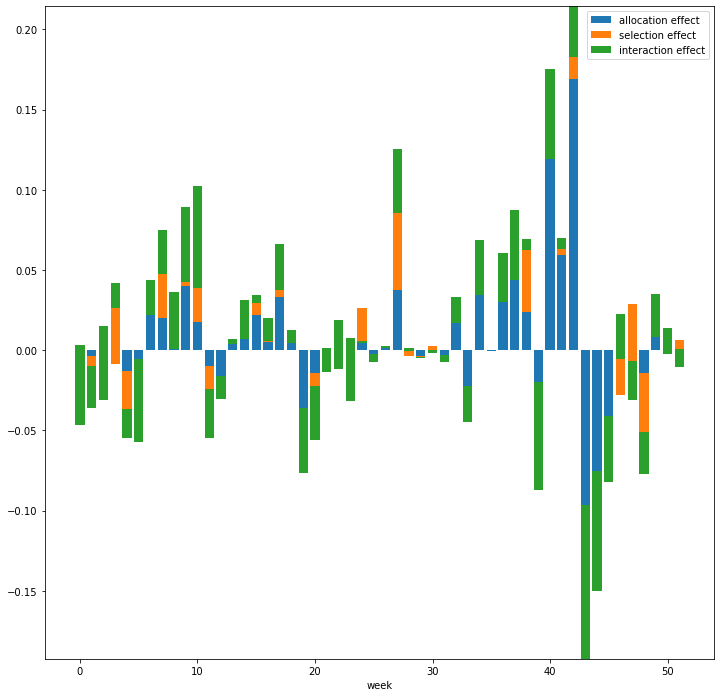

Finally, we draw the average effects on each sector.

[# brinson sector analysis
brinson_sector_analysis = pd.DataFrame()

brinson_sector_analysis['sector'] = brinson_model.sector.unique()
brinson_sector_analysis['allocation_effect'] = np.nan
brinson_sector_analysis['selection_effect'] = np.nan
brinson_sector_analysis['interaction_effect'] = np.nan
brinson_sector_analysis['excess_return'] = np.nan


for i in range(len(brinson_model.sector.unique())):
  s = brinson_model.sector.unique()[i]
  allocation_effect = brinson_model[brinson_model.sector==s].allocation_effect.mean()
  selection_effect = brinson_model[brinson_model.sector==s].selection_effect.mean()
  interaction_effect = brinson_model[brinson_model.sector==s].interaction_effect.mean()
  excess_return = brinson_model[brinson_model.sector==s].excess_return.mean()
  
  brinson_sector_analysis['allocation_effect'][i] = round(allocation_effect,5)
  brinson_sector_analysis['selection_effect'][i] = round(selection_effect,5)
  brinson_sector_analysis['interaction_effect'][i] = round(interaction_effect, 5)
  brinson_sector_analysis['excess_return'][i] = round(excess_return, 5)

pole = brinson_sector_analysis.sector.unique()
 
# Initialise the spider plot by setting figure size and polar projection
plt.figure(figsize=(15, 12))
plt.subplot(polar=True)
 
theta = np.linspace(0, 2 * np.pi, len(pole))
 
# Arrange the grid into number of sales equal parts in degrees
lines, labels = plt.thetagrids(range(0, 360, int(360/len(pole))), (pole), fontproperties=zhfont, fontsize=15)
 
# Plot actual sales graph
plt.plot(theta, (brinson_sector_analysis.allocation_effect*100).to_list())
plt.plot(theta, (brinson_sector_analysis.selection_effect*100).to_list())
plt.plot(theta, (brinson_sector_analysis.interaction_effect*100).to_list())
 
# Add legend and title for the plot
plt.legend(labels=('allocation effect', 'selection effect', 'interaction effect'), loc=0, fontsize=8)
plt.title("average effect by sector (%)", fontsize=20)
 
plt.show()](https://i.postimg.cc/ZK5TPpjD/3.png)

Voila!!!