A Geobase quickstart blueprint application showing animated taxis movements with h3 grid analysis


- What's included
- Prerequisites
- Development
- Using The App
- Deployment
- Database Overview
- Video
- Learn More
- Further Info
- Authors
This is a Geobase & React application that shows animated taxi trips on a map around the city of Porto, Portugal. It uses the powerful PostgreSQL extensions MobilityDb, H3 and PostGIS, all built into Geobase, with MapLibre and deck.dl on the webpage. The application can also interactively query the data to calculate aggregate statistics. In addition, the data is processed to display "close passes" where two taxis pass by each other in time and space. With just minimal editing, a user can quickly get started loading, processing and viewing dynamic temporal geospatial data.
The data is from 2013 which contains GPS trajectories of taxis in Porto, Portugal. The dataset includes information such as taxi IDs, timestamps, and GPS coordinates (latitude and longitude) for each trip. This quickstart will import, processes and make the data available as temporal vector tiles. The vector tiles are then displayed using Deck.gl on a Maplibre map. Users can perform a query to view trip statistics as 3D hexagons displayed on the map via a database function.
The first step is to have an account on Geobase and to create a new project.
It's good to have basic familiarity with running PostgreSQL psql commands, Node or running e.g React applications (e.g. via nvm and using npm)
Once you're Geobase project is created, you can manually download, clone or create a new GitHub repository using this template by clicking here. This will create a copy of this repo without the git history.
First you will need to load and process the data for the application. You can run SQL from within the Geobase application, or you connect from your own system. It's probably a good idea to read the SQL files to see what it's going to do before you run it. There are a few steps to load and process the data.
Step 1: Set the geobase database URI
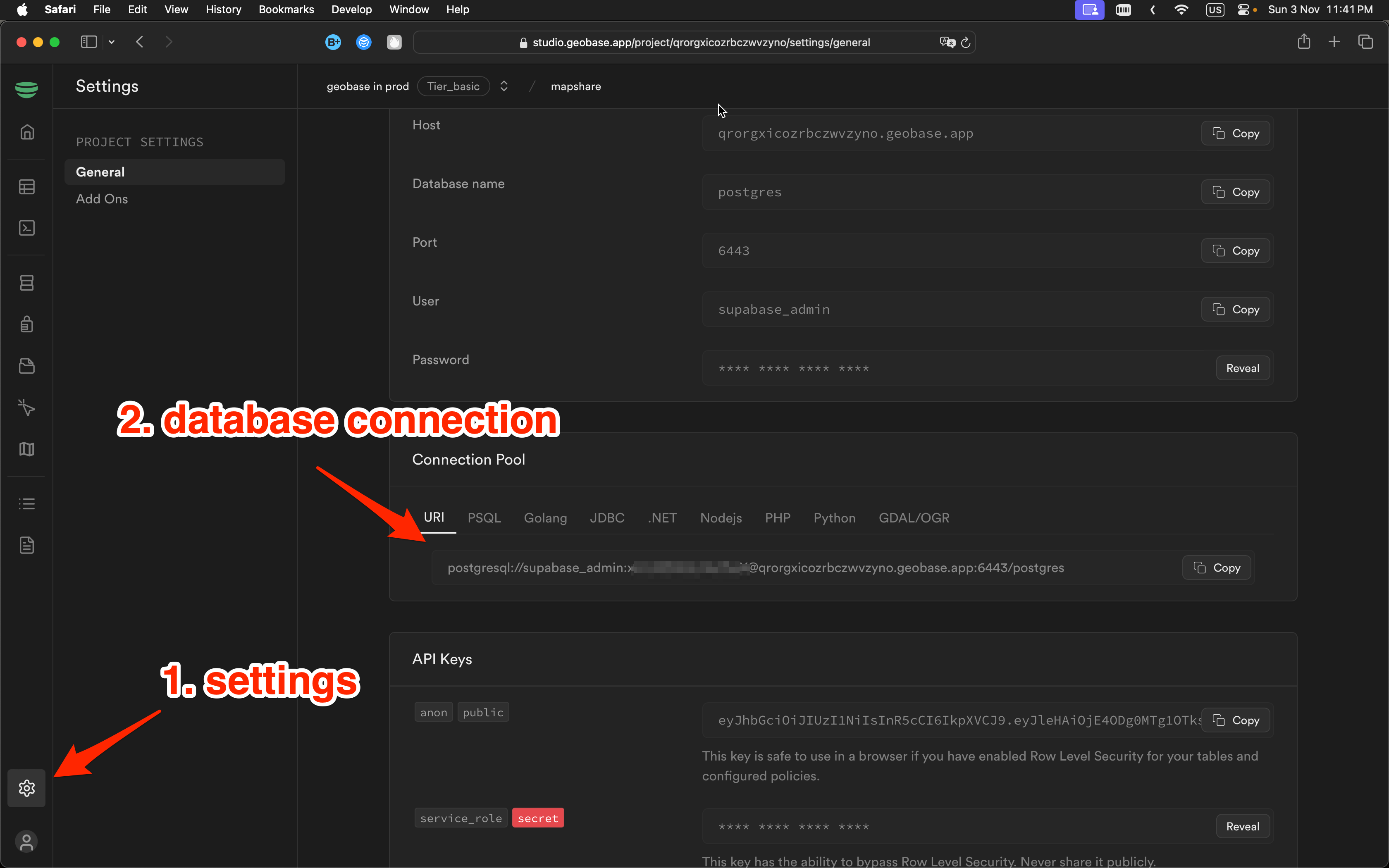
Set the database uri in your environment, you can get it from the Geobase project settings page:
# set the database uri in your environment
DATABASE_URI=<your-database-uri>
Step 2: Set up tables
psql -d $DATABASE_URI -f geobase/1setup.sqlStep 3: Unzip the file geobase/taxis_2k.zip to extract the CSV file train_2k.csv. This file contains the 2,000 taxi trips. You can use a command like this:
unzip geobase/taxis_2k.zip -d geobaseStep 4: From your local terminal, load in the data into the taxis_staging table. This may take a few seconds depending on the network speed and the size of the file.
Load the data into the taxis_staging table using the \copy command:
psql -d $DATABASE_URI -c "\copy taxis_staging FROM 'geobase/train_2k.csv' WITH (FORMAT csv, HEADER true, DELIMITER ',')"Step 5: Convert and clean the data and create the functions. This step may take the longest depending on the size of the tables as there is some processing and cleaning involved, explained below
psql -d $DATABASE_URI -f geobase/2convert.sqlTo connect your app to Geobase, configure these environment variables. Include them in a .env.local file for local development. You can copy and rename the .env.example given in the repository and edit it.
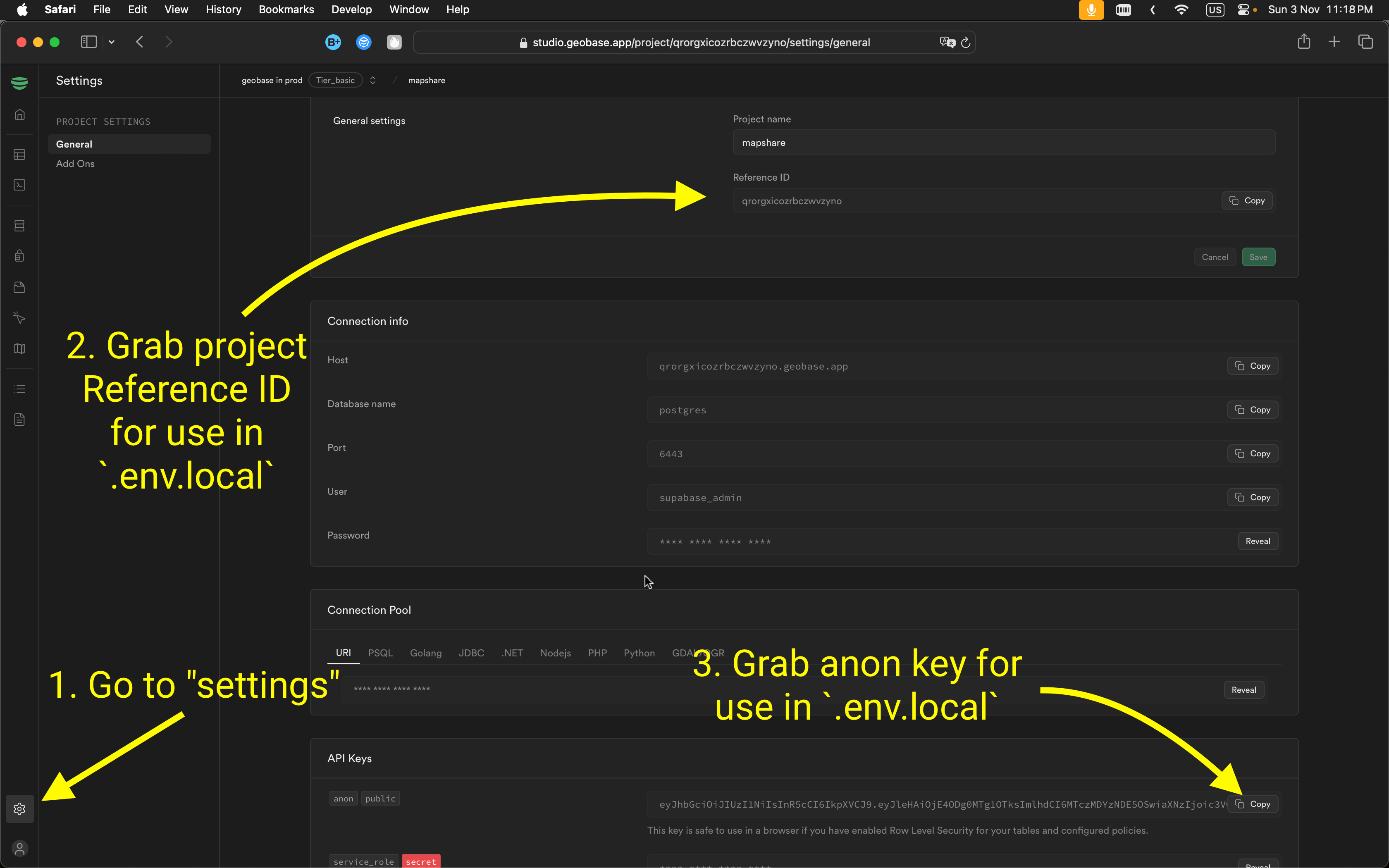
VITE_GEOBASE_URL=https://YOUR_PROJECT_REF.geobase.app
VITE_GEOBASE_ANON_KEY=YOUR_GEOBASE_PROJECT_ANON_KEY
You can find the project ref and anon key in the Geobase project settings page:
Use nvm to set node version, e.g.
nvm use 21Install dependencies:
npm install
# or
pnpm install
Run dev:
npm run dev
# or
pnpm run dev
Open http://localhost:5173 with your browser to see the blueprint in action.
You should see a page with a map showing the animated taxi trips. It should show something like this animation:

You can start and stop the animation using the timeline control below the map. You can grab the timeline slider manually to scrub backwards and forwards in time, and the map display will change.
If you have loaded in the 2000 taxi trips, the time range for the trips starts after midnight, goes through the morning rush hour and ends around lunchtime when there is a quiet period. You can see trips going to and from the airport and to and from the train stations and from taxi stands.
You should see the taxis trips styled with 3 colours: Red trips are trips that were dispatched from the central office, green trips are trips that left a designated taxi stand, and blue trips are taxi rides rides that were hailed in the street and other uncategorized trips.
The pulsing light blue circles on the map represent areas where two taxis have passed each other in time and space within a 10m distance.
To view statistics about the taxi trips on hexagon polygon map layer, you can enter the start time and end time and choose the statistics to display for the colour (or fill) or the hexagon and for the height (or elevation) of the hexagon. Depending on the time range you choose, and the amount of data in your tables, the query may take a few seconds to complete. You can mouse over the hexagons to see the statistics for that hexagon displayed in a tooltip. To clear this hexagon statistics layer, click the "Clear Stats Layer" button, or press the "Escape" key.

For the specified time range, the statistics are:
- Trip count: The total number of taxi trips that pass within the hexagon.
- Average duration: The average duration, in seconds, of taxi trips that pass within the hexagon.
- Average speed in the area: The average speed, in km/h, of taxi trips within this hexagon.
- Average speed of trips across: The average speed, in km/h, of taxi trips that pass through this hexagon. (i.e. whats the average speed of all the journeys that go into and out of this area)
- Speed difference: The difference between the speed within this specific area and across the entire journey. We can get an indication if this area is slower or faster compared to other areas.
One easy way to deploy this blueprint app is to use the Vercel Platform from the creators of Next.js. Check out the Next.js deployment documentation for more details.
A good summary of how the database is setup can be found in the two sql files in the geobase folder; geobase/1setup.sql and geobase/2convert.sql. These files set up a number of tables, indexes and functions.
The database migrations sets up the following tables and functions. See Learn More below for more details about the cleaning, analysis and methods used.
taxis_staging: This table is used to import the raw taxis data from the CSV file. 2000 rows. This table is dropped later on..taxis_cleaning: This table is used to clean and convert the taxis_staging data. This table is dropped later on.taxis: The final taxi trips table used for analysis and maps. 1962 rows. This is created from the taxis_cleaning table by using mobilitydb operations to find and remove outliers - periods of time where the speed was impossibly high.hexgrid: A table of H3 hexagon polygons, clipped to the extent of the taxis table.closest_taxis_points: Table created from analyzing the taxis table to find which trips pass by each other within a 10 metres distance.
public.taxis_fn(): Create vector tiles (mvt) with embedded timestamps, to be served by the Geobase tile server. This function powers the animated taxi movements on the map.public.get_hex_trip_metrics_for_period(analysis_period): Queries each hexagon in thehexgridfor all the trips in thetaxistable, calculating and aggregating a range of statistics.public.get_taxis_time_range_fn(): Returns the time range of the taxis data. E.g. the min and max timestamp.
The get_taxis_time_range_fn function sets up the interface to work with the full range of the data in your tables. If you wish to manually set the time range, you can edit the start_time and end_time variables within the src/lib/consts.ts file e.g.
export const STATIC_TIME_RANGE = {
  start_time: "2013-07-01 08:00:20+00",
  end_time:   "2013-07-01 12:30:20+00"
};Row Level Security is implemented for the tables to ensure data privacy and access control.
Enable read access for all users is enabled for for taxis and for closest_taxis_points. This enables the tables to be shown on the map or viewed in a desktop GIS for further querying.

🎥 Take a look at the blueprint overview video on YouTube
The data originated from a challenge at the European Conference on Machine Learning and Principles and Practice of Knowledge Discovery in Databases Conference, held in Portugal in 2015. The data is published at Taxi Trajectory Prediction on Kaggle and also Taxi Trajectory Data on Kaggle which has more information about the format of the data. In it's full version, the data spans a whole year (from July 2013 to July 2014) for all 442 taxis in the city. In this quickstart we have just taken the first 2000 rows of this huge csv file which cover around 12 hours, from midnight to lunchtime on 1 July 2013.
MobilityDB is an extension of PostgreSQL and PostGIS that provides temporal types, for example a moving vehicle, recording it's speed and position. In this quickstart we use the temporal point type tgeompoint and a sequence of such points creates a tgeompointSeq - conceptually a linestring of temporal points. More detail about the use of mobilitydb and functions are given below.
A temporal sequence point (tgeompointSeq) represents a continuous movement between spatial positions over time. The function trajectory extracts the spatial path of this movement as a PostGIS linestring geom. The trajectory is used with a spatial index to speed up bounding box intersection queries.
In the taxis_fn, we want to include timestamps with our trips on the map. We use the MobilityDB function asMVTGeom to return the line string geometries and times attributes based on the passed in bounds geometry. The taxis_fn function, to speed up queries, does a bounding box overlap operation && of the linestring trajectory of the trip with the requested tile bounds.
Geobase has the h3 postgres extension built in. H3 is a geospatial indexing that uses a hexagonal grid which can be subdivided into progressively finer hexagonal grids. The h3 extension is used to create the hexgrid table.
The taxis_staging table is cleaned and processed. Starting with 2000 rows, 61 rows are removed.
After creation, it is processed. First we convert the coordinate strings into PostGIS geometries and the timestamp string is converted into a database timestamp object. Next, a few features are filtered where the length is too short, or where the trips are marked as having "missing data". Finally, a MobilityDB tgeompoint type (temporal_geom) is created. Each point in the line string was recorded at a 15 second interval so we can construct the time of each point from the starting timestamp.
The taxis csv file contains rows like the following:
"TRIP_ID","CALL_TYPE","ORIGIN_CALL","ORIGIN_STAND","TAXI_ID","TIMESTAMP","DAY_TYPE","MISSING_DATA","POLYLINE"
"1372636858620000589","C","","","20000589","1372636858","A","False","[[-8.618643,41.141412],[-8.618499,41.141376], ... ,[-8.630838,41.154489]]"
The taxis_staging table is processed into the taxis_cleaning table, removing some columns in the process.
The polyline coordinate strings are converted into PostGIS geometries line_geom:
ST_SetSRID(ST_GeomFromGeoJSON('{"type":"LineString","coordinates":' || polyline || '}'), 4326)
and the timestamp string is converted into a timestamp object. Some rows are deleted where the length of the geometries are less than 4 st_numpoints(line_geom) < 4 This ensures that we see actual lines.
Let us look at the creation of the tgeompoint MobilityDB temporal point type into temporal_geom:
UPDATE taxis_cleaning
SET temporal_geom = (
    SELECT tgeompointSeq(
        array_agg(
            tgeompoint(
                ST_PointN(ST_Transform(line_geom, 3857), point_num),
                t + (point_num - 1) * INTERVAL '15 seconds'
            )
        )
    )
    FROM generate_series(1, ST_NPoints(line_geom)) AS point_num
);
We know that each point in the line was recorded at 15 seconds intervals, and we only have the timestamp when the trip was first started. This then loops over the point vertices in the line_geom and creates a tgeompoint( point, time ) for each point. The projection of the line_geom attribute is in EPSG:4326 (e.g. latitude and longitude) so we need to reproject it using ST_Transform(line_geom, 3857), into EPSG:3857 (e.g. web mercator using metres). Then we make a tgeompointseq a sequence of temporal points, representing the trip line.
For details on how to connect Geobase to QGIS or other desktop GIS software, have a look at the A Guide to Connecting QGIS and Geobase for GIS Analysts in the Geobase documentation.
Looking at taxis_cleaning.line_geom in QGIS shows a number of outliers - long lines that jump out from a trip and cross almost the entire map.

As we know each point along the line is taken at 15 seconds intervals, if a section between two points is a large distance, we know that the speed of that part is going to be very high. By removing periods where the speed is unrealistic, we clean these outliers from the data within the geobase/2convert.sql file.

The identification of high speed periods is facilitated by:
whenTrue(speed(temporal_geom) #> 55) AS high_speed_periods
whenTrue is a MobilityDB function which returns the time when a temporal boolean is true.
speed is a MobilityDB function which returns the speed of the temporal point in units (metres) per second. The statement speed(temporal_geom) #> 55) returns a true or false boolean. high_speed_periods is therefore the periods in a trip which need to be removed.
The removal of these periods is done by:
  WHEN high_speed_periods IS NOT NULL THEN
    minusTime(temporal_geom, spanset(span(high_speed_periods)))
  ELSE
    temporal_geom
minusTime is a MobilityDB function that restricts to the complement of a time value. This means it restricts the trip to every point except the passed in time value. spanset(span(high_speed_periods))) is used to group the periods we want to delete together into one spanset.
Here is an image showing before and after the cleaning process. From around 2000 trips, 280 had outliers that were cleaned.

For these 280 trips, as what might have been one continuous line may now be broken to remove the outliers, we can construct our PostGIS geometry using a few functions. We also ensure that any Linestrings from rows that didn't have any outliers are also turned into MultiLineStrings, as we want all the rows to have the same type of geometry.
geom = ST_Multi(ST_CollectionExtract(trajectory(cleaned_temporal_geom), 2))trajectory is a MobilityDB function that returns the PostGIS geometry trajectory of the tgeompoint, this may be a collection of geometries, a collection of lines.
ST_CollectionExtract is the PostGIS function that creates Linestring multi geometry (MultiLineString) from the passed in geometry objects.
ST_Multi is a postGIS function that returns the geometry as a MultiLineString.
The function public.get_hex_trip_metrics_for_period(analysis_period tstzspan) which you can view within the geobase/2convert.sql file uses a few MobilityDB functions to calculate stats.
For the passed in analysis_period time span and for each hexagon polygon in hexgrid it calculates a range of statistics such as the duration and speed of trips within each polygon.
SELECT
    h.h3,
    COUNT(*) AS trip_count,
    AVG(EXTRACT(EPOCH FROM duration(clipped_geom))) AS avg_duration_seconds,
    AVG(twavg_speed) AS avg_speed_in_ms,
    AVG(all_twavg_speed) AS avg_speed_in_ms_all_hex
FROM hexgrid h,
     LATERAL (
         SELECT
             -- Clip the trajectory to both the hexagon and the time period
             atGeometry(attime(t.cleaned_temporal_geom, analysis_period), h.geom) AS clipped_geom,
             twavg(speed(atGeometry(attime(t.cleaned_temporal_geom, analysis_period), h.geom))) AS twavg_speed,
             twavg(speed(attime(t.cleaned_temporal_geom, analysis_period))) AS all_twavg_speed
         FROM taxis t
         WHERE
             -- Filter trips that spatially and temporally intersect and which have a duration bigger than 0
             t.geom && h.geom
             AND (t.cleaned_temporal_geom::tstzspan) && analysis_period
             AND duration(atGeometry(attime(t.cleaned_temporal_geom, analysis_period), h.geom)) > INTERVAL '0 seconds'
     ) AS trip_data
GROUP BY h.h3
ORDER BY trip_count DESC;
Lets look at some of these in more detail:
Passing in the time range and hexagon geometry, this returns a temporally and spatially clipped temporal geometry.
twavg(speed(atGeometry(attime(t.cleaned_temporal_geom, analysis_period), h.geom))) AS twavg_speed
atTime similar to minusTime used above, returns the trips only for the specific time.
atGeometry restricts the temporal geometry to the hexagon polygon geometry.
twavg returns the time weighted average of the speed of the temporal geometry within this polygon.
The following returns the average duration in seconds from the trips within the area within the time period:
AVG(EXTRACT(EPOCH FROM duration(clipped_geom))) AS avg_duration_seconds,To speed up the query, the where clause in the function has a few statements worth looking at:
t.geom && h.geom
The && is a PostGIS bounding box operator It enables the function to only calculate statistics that intersect the bounding box of the hexagon.
(t.cleaned_temporal_geom::tstzspan) && analysis_period
This is a temporal intersection, making sure that it only runs on temporal geometries that occur within the selected time range.
duration(atGeometry(attime(t.cleaned_temporal_geom, analysis_period), h.geom)) > INTERVAL '0 seconds'This statement finally ensures that the trip within the hexagon has a duration. In other words, it's another check to ensure that it's a actual trip.
Note, as this function may take a few seconds to query, depending on the size of the data in the tables, time range requested and performance of the database, to be on the safe side we increase the statement_timeout setting.
ALTER ROLE anon SET statement_timeout = '15s';
NOTIFY pgrst, 'reload config';
The closest_taxis_points table is created by evaluating trips with each other and seeing which ones pass within 10 metres of each other.
SELECT startTimestamp(atMin(t1.cleaned_temporal_geom <-> t2.cleaned_temporal_geom)),
       valueAtTimestamp(t2.cleaned_temporal_geom, startTimestamp(atMin(t1.cleaned_temporal_geom <-> t2.cleaned_temporal_geom)))
FROM taxis t1, taxis t2
WHERE t1.trip_id > t2.trip_id
  AND edwithin(t1.cleaned_temporal_geom, t2.cleaned_temporal_geom, 10);
edwithin(geom1, geom2, distance) returns true or false if the two geometries are ever within the specified distance.
valueAtTimestamp returns a point at the specified timestamp.
startTimeStamp this simply returns the first timestamp of the trip
atMin restricts the trip to the minimum value of (t1.cleaned_temporal_geom <-> t2.cleaned_temporal_geom)
The mobilitydb temporal distance operator, <->, computes the distance at each instant of the intersection of each trip and results in an array of distance and the timestamp of that distance (e.g. 0.7451@2001-01-03 08:10). So we have an array of times when the trips are closest to each other within the 10m, and we can get the minimum of that array.
So putting it together we get the point and the timestamp of that point, where the closest distance between two trips is measured.
Here is a screenshot of the taxi trips and the closest pass points:

You can see that most close passes happened on the major roads, but there are some on some minor ones.
MapLibre is the mapping library used and provides the basemap style.
Deck.gl is a WebGL-powered framework for visual exploratory data analysis of large datasets. It is used with maplibre to render the vector tiles, the animated trails and the close passes on the map.
A vector linestring feature from the tile server has an array of coordinates and a timestamps property. For example:
{
  "type": "Feature",
  "geometry": {
    "type": "LineString",
    "coordinates": [
      [ 15.04302, 54.13267 ],
      [ 15.09658, 53.91566 ],
      [ 15.14739, 53.69995 ],
      [ 15.18173, 53.54438 ]
    ]
  },
  "properties": {
    "call_type": "A",
    "trip_id": 123,
    "timestamps": [1610064000,1610064072,1610064142,1610064192],
  }
}
The Deck.gl MVTLayer loads in the layer for the taxis and the renderSubLayers prop is called for each tile so that for each tile a TripsLayer tile is returned. This TripsLayer reads the data of the feature for getPath (the coordinates) and getTimestamps (the timestamps array).
For the closest pass animations, a Deck.gl MVTLayer is loaded with renderSubLayers and a ScatterplotLayer is called for each tile. The ScatterplotLayer renders circles at specified positions. The way the points are hidden, shown and fade are due to the getFillColor function and the growing animation with the getRadius function.
getFillColor: d => {
  const pointTime = Math.floor(new Date(d.properties.time_at_closest).getTime() / 1000) - minTimestamp;
  const duration = 400; // Duration to show each point

  // is it visible now?
  if (currentTime >= pointTime && currentTime <= pointTime + duration) {
    // Fade effect based on age
    const age = currentTime - pointTime;
    const opacity = Math.max(0, 255 * (1 - age / duration));
    return [105, 174, 255, opacity]; // fade the colour
  }

  return [0, 0, 0, 0]; // Invisible
},
The getFillColor function evaluates if the point should be visible or not by looking at the currentTime (changed by the timeline) and the time of the point. If it should not be visible, it returns an invisible point, and if it is visible, depending on the time passed, it will change the colour to make it fade.
Finally, updateTriggers is defined. This enables Deck.gl to re-evaluate the getFillColor and getRadius based on when an external variable changes (currentTime). By using this it's better for performance than updating the layer fully each time.
updateTriggers: {
    getFillColor: [currentTime],
    getRadius: [currentTime]
  }
For additional information, refer to:
For support, reach out on the Geobase Discord.