Basics of RDkit

The Rdkit supports conda installation

conda -c rdkit rdkit

Installing the libraries

pip install useful_rdkit_utils requests pandas sklearn tqdm numpy seaborn mols2grid matplotlib

Import the necessary python libraries

from rdkit import Chem 
from rdkit.Chem.Draw import IPythonConsole 
from rdkit.Chem import Draw 

from rdkit.Chem import rdDepictor
IPythonConsole.ipython_useSVG = True
rdDepictor.SetPreferCoordGen(True)
from rdkit.Chem import PandasTools 
import mols2grid 
import requests

Displaying a chemical structure from the SMILES string

mol=Chem.MOLFromSmiles(c1ccccc1)
mol

Converting RDKit molecule to SMILES python

smi=Chem.MolToSmiles(mol)
smi

'c1ccccc1'

Moreover we can convert RDkit molecule to InchiKey Replacing Smiles by InchiKey.

Chem.MolToInchiKey(mol)

'UHOVQNZJYSORNB-UHFFFAOYSA-N'

PS: You can get the smiles string of almost every drug available from wikipedia. But you need to have basics understainding of how to represents the structure in SMILES form. Refer [https://archive.epa.gov/med/med_archive_03/web/html/smiles.html] for basics of SMILES and [https://www.rdkit.org/docs/GettingStartedInPython.html#reading-sets-of-molecules] for RDKit.

Clustering the structures using K-means algorithm

Install the python Libraries

pip install useful_rdkit_utils pandas sklearn tqdm numpy seaborn mols2grid matplotlib

Import the necessary Python Libraries

import pandas as pd
import useful_rdkit_utils as uru
from rdkit import Chem
from sklearn.cluster import KMeans
from sklearn.metrics import silhouette_score, silhouette_samples
from tqdm.auto import tqdm
import numpy as np
import seaborn as sns
from sklearn.manifold import TSNE
import mols2grid
import matplotlib.cm as cm

Read the input data

smiles_url = "https://raw.githubusercontent.com/PatWalters/practical_cheminformatics_tutorials/main/data/cluster_test.smi"
df = pd.read_csv(smiles_url,sep=" ",names=["SMILES","Name"])

I made this note with the help of tutorial by Pat Walters. If you want to know more about RDkit follow his blog [https://practicalcheminformatics.blogspot.com/] and github [https://github.com/PatWalters/practical_cheminformatics_tutorials]

The file df looks like (df.head())

SMILES	Name
0	CCC(=O)/N=C1\S[C@H]2CS(=O)(=O)C[C@@H]2N1c1ccc(...	16741133
1	Cc1ccc(Cl)cc1N1/C(=N\C(=O)CCC(=O)O)S[C@H]2CS(=...	101303273
2	CCCCC(=O)/N=C1/S[C@H]2CS(=O)(=O)C[C@@H]2N1c1cc...	32504126
3	CCN(CC)c1ccc(N2/C(=N\C(=O)CC#N)S[C@H]3CS(=O)(=...	101319242
4	CC[C@H](C)C(=O)/N=C1/S[C@H]2CS(=O)(=O)C[C@H]2N...	36638719

Add molecules fingerprints

df['mol']=df.SMILES.progress_apply(Chem.MolFromSmiles)
df['fp']=df.mol.progress_apply(uru.mol2morgan_fp]

df.head()

0	CCC(=O)/N=C1\S[C@H]2CS(=O)(=O)C[C@@H]2N1c1ccc(...	16741133	<rdkit.Chem.rdchem.Mol object at 0x7f426506c6c0>	[0, 0, 0, 0, 0, 0, 0, 0, 0, 0, 0, 0, 0, 0, 0, ...
1	Cc1ccc(Cl)cc1N1/C(=N\C(=O)CCC(=O)O)S[C@H]2CS(=...	101303273	<rdkit.Chem.rdchem.Mol object at 0x7f426506c9e0>	[0, 0, 0, 0, 0, 0, 0, 0, 0, 0, 0, 0, 0, 0, 0, ...
2	CCCCC(=O)/N=C1/S[C@H]2CS(=O)(=O)C[C@@H]2N1c1cc...	32504126	<rdkit.Chem.rdchem.Mol object at 0x7f426506c760>	[0, 0, 0, 0, 0, 0, 0, 0, 0, 0, 0, 0, 0, 0, 0, ...
3	CCN(CC)c1ccc(N2/C(=N\C(=O)CC#N)S[C@H]3CS(=O)(=...	101319242	<rdkit.Chem.rdchem.Mol object at 0x7f426506cbc0>	[0, 0, 0, 0, 0, 0, 0, 0, 0, 0, 0, 0, 0, 0, 0, ...
4	CC[C@H](C)C(=O)/N=C1/S[C@H]2CS(=O)(=O)C[C@H]2N...	36638719	<rdkit.Chem.rdchem.Mol object at 0x7f426506ca30>	[0, 1, 0, 0, 0, 0, 0, 0, 0, 0, 0, 0, 0, 0, 0, ...

Convert to matrix

X=np.satck(df.fp)

X

array([[0, 0, 0, ..., 0, 0, 0],
       [0, 0, 0, ..., 0, 0, 0],
       [0, 0, 0, ..., 0, 0, 0],
       ...,
       [0, 0, 0, ..., 0, 0, 0],
       [0, 0, 0, ..., 0, 0, 0],
       [0, 0, 0, ..., 0, 0, 0]])
       ```
       
Lets start clustering now

```num_clusters=10
km = KMeans(n_clusters=num_clusters,random_state=42)
km.fit(X)
cluster_list = km.predict(X)

plot the cluster population

ax = pd.Series(cluster_list).value_counts().sort_index().plot(kind="bar")
ax.set_xlabel("Cluster Number")
ax.set_ylabel("Cluster Size")
ax.tick_params(axis='x', rotation=0)

Here we do not know the range of the clusters the only thoing that we can do is guess. The way of determining the optimal number of clusters is by minimising the silhouette score [https://en.wikipedia.org/wiki/Silhouette_(clustering)]

Sillhoutte Score = $(a-b)$/$max(a,b)$

cluster_range = range(2,30)
score_list = []
for k in tqdm(cluster_range):
    km = KMeans(n_clusters=k,random_state=42)
    cluster_labels = km.fit_predict(X)
    score = silhouette_score(X,cluster_labels)
    score_list.append([k,score])

You can use any range (see cluster_range=range(2,30) but be careful about the range, you will end up with almost the same minima. Put the scores in DataFrame

 score_df = pd.DataFrame(score_list,columns=["K","Silhouette Score"])
score_df.head()

K	Silhouette Score
0	2	0.171716
1	3	0.242523
2	4	0.280316
3	5	0.311763
4	6	0.332428

plot the scores

ax = sns.lineplot(x="K",y="Silhouette Score",data=score_df)
ax.set_xticks(cluster_range)

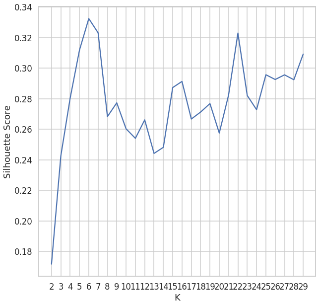
Count the minima from the above figure (=14) So there are 14 different clusters. Lets make it 14 now.

num_clusters = 14
km_opt = KMeans(n_clusters=num_clusters)
clusters_opt = km_opt.fit_predict(X)

plot

def silhouette_plot(X,cluster_labels):
    """
    Adapted from https://scikit-learn.org/stable/auto_examples/cluster/plot_kmeans_silhouette_analysis.html
    """
    sns.set_style('whitegrid')
    sample_df = pd.DataFrame(silhouette_samples(X,cluster_labels),columns=["Silhouette"])
    sample_df['Cluster'] = cluster_labels
    n_clusters = max(cluster_labels+1)
    color_list = [cm.nipy_spectral(float(i) / n_clusters) for i in range(0,n_clusters)]
    ax = sns.scatterplot()
    ax.set_xlim([-0.1, 1])
    ax.set_ylim([0, len(X) + (n_clusters + 1) * 10])
    silhouette_avg = silhouette_score(X, cluster_labels)
    y_lower = 10
    unique_cluster_ids = sorted(sample_df.Cluster.unique())
    for i in unique_cluster_ids:
        cluster_df = sample_df.query('Cluster == @i')
        cluster_size = len(cluster_df)
        y_upper = y_lower + cluster_size
        ith_cluster_silhouette_values = cluster_df.sort_values("Silhouette").Silhouette.values
        color = color_list[i]
        ax.fill_betweenx(np.arange(y_lower, y_upper),
                    0, ith_cluster_silhouette_values,
                    facecolor=color, edgecolor=color, alpha=0.7)
        ax.text(-0.05, y_lower + 0.5 * cluster_size, str(i),fontsize="small")
        y_lower = y_upper + 10
    ax.axvline(silhouette_avg,color="red",ls="--")
    ax.set_xlabel("Silhouette Score")
    ax.set_ylabel("Cluster")
    ax.set(yticklabels=[]) 
    ax.yaxis.grid(False) 
silhouette_plot(X,clusters_opt)

Clustered plot

tsne = TSNE(n_components=2, init='pca',learning_rate='auto')
crds = tsne.fit_transform(X,clusters_opt)
color_list = [cm.nipy_spectral(float(i) / num_clusters) for i in range(0,num_clusters)]
ax = sns.scatterplot(x=crds[:,0],y=crds[:,1],hue=clusters_opt,palette=color_list,legend=True)
ax.legend(loc='upper left', bbox_to_anchor=(1.00, 0.75), ncol=1);

Display the clusters molecules (members)

cluster_id = 1
cols = ["SMILES","Name","Cluster"]
display_df = opt_cluster_df[cols].query("Cluster == @cluster_id")
mols2grid.display(display_df,subset=["img"],n_cols=3,size=(320,240))

All these scripts are from [https://github.com/PatWalters/practical_cheminformatics_tutorials] You can easily access it from there and run those scripts in google colab. Many Thanks to Pat Walters.